Other useful Python packages#

Announcements#

CAPES and survey available!
- Survey: https://forms.gle/xox1KgV6FwCYoESX6
- CAPES: https://cape.ucsd.edu/student/instructions.html

Goals of this lecture#

Review of course: what we’ve learned this quarter.
Overview of other useful Python packages:
- seaborn: easily and quickly make data visualizations.
- scipy: tools for statistical analyses.
- nltk: tools for Natural Language Processing, like sentiment analysis.

What we’ve learned#

Reflect on the very first day of class: most of you had never programmed before!
Now you know:
- How to use Jupyter notebooks.
- How to write if statements and for loops.
- How to create custom functions.
- How to read in files of various types.
- How to work with tabular data using pandas.

That’s a lot for ten weeks!

Data visualization with `seaborn`#

What is data visualization?#

Data visualization refers to the process (and result) of representing data graphically.

CSS 2 will dedicate much more time to this.
Today: introduction to seaborn.

import matplotlib.pyplot as plt # conventionalized abbreviation
import pandas as pd
import seaborn as sns
%matplotlib inline 
%config InlineBackend.figure_format = 'retina'

/opt/anaconda3/lib/python3.9/site-packages/scipy/__init__.py:146: UserWarning: A NumPy version >=1.16.5 and <1.23.0 is required for this version of SciPy (detected version 1.26.2
  warnings.warn(f"A NumPy version >={np_minversion} and <{np_maxversion}"

Example dataset#

## Load taxis dataset
df_taxis = sns.load_dataset("taxis")
len(df_taxis)

df_taxis.head(2)

	pickup	dropoff	passengers	distance	fare	tip	tolls	total	color	payment	pickup_zone	dropoff_zone	pickup_borough	dropoff_borough
0	2019-03-23 20:21:09	2019-03-23 20:27:24	1	1.60	7.0	2.15	0.0	12.95	yellow	credit card	Lenox Hill West	UN/Turtle Bay South	Manhattan	Manhattan
1	2019-03-04 16:11:55	2019-03-04 16:19:00	1	0.79	5.0	0.00	0.0	9.30	yellow	cash	Upper West Side South	Upper West Side South	Manhattan	Manhattan

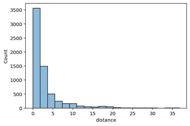
Histograms#

Histograms are critical for visualizing how your data distribute.
Used for continuous variables.

sns.histplot(data = df_taxis, x = "distance", alpha = .5, bins = 20)

<AxesSubplot:xlabel='distance', ylabel='Count'>

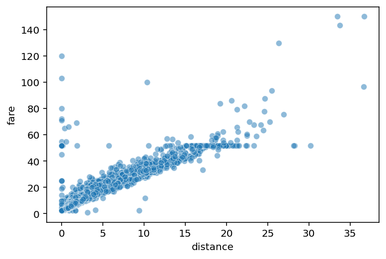
Scatterplots#

Scatterplots are useful for visualizing how two continuous variables relate.

sns.scatterplot(data = df_taxis, x = "distance", 
                y = "fare", alpha = .5)

<AxesSubplot:xlabel='distance', ylabel='fare'>

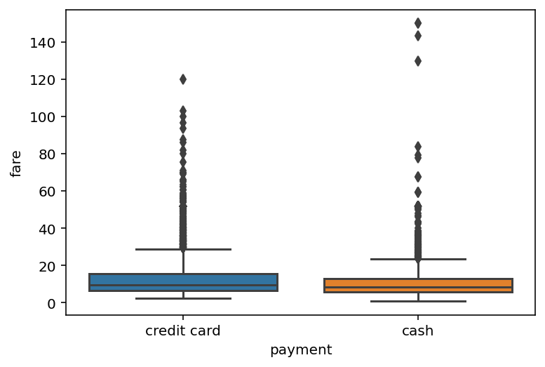
Boxplots#

Boxplots are useful for visualizing one continuous variable as it relates to a categorical variable.

sns.boxplot(data = df_taxis, 
            x = "payment", 
            y = "fare")

<AxesSubplot:xlabel='payment', ylabel='fare'>

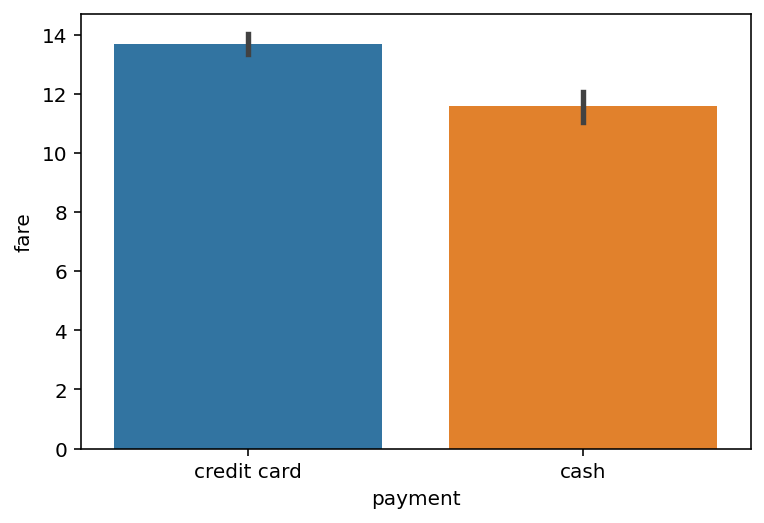
Barplots#

Barplots are also useful for visualizing one continuous variable as it relates to a categorical variable.
Typically less informative than a boxplot or violinplot.

sns.barplot(data = df_taxis, 
            x = "payment", 
            y = "fare")

<AxesSubplot:xlabel='payment', ylabel='fare'>

Statistics with `scipy`#

scipy is a Python package with many uses, including statistics.

import scipy.stats as ss

Calculating correlations#

scipy.stats can be used to calculate a correlation coefficient.

## Gives correlation between distance and fare
ss.pearsonr(df_taxis['distance'],
           df_taxis['fare'])

(0.9201077027895823, 0.0)

Comparing to visualization#

Consistent with correlation coefficient: strong, positive relationship between fare and distance.

sns.scatterplot(data = df_taxis, x = "distance", 
                y = "fare", alpha = .5)

<AxesSubplot:xlabel='distance', ylabel='fare'>

Running a t-test#

A t-test compares two samples: how likely is it that these two samples came from the same “population”?

sns.barplot(data = df_taxis, 
            x = "payment", 
            y = "fare")

<AxesSubplot:xlabel='payment', ylabel='fare'>

t-test in `scipy`#

## First, filter our data to get cash vs. credit
cash = df_taxis[df_taxis['payment'] == 'cash']
credit = df_taxis[df_taxis['payment'] == 'credit card']

## Now, run t-test comparing fare for cash vs. credit
## Very significant p-value
ss.ttest_ind(credit['fare'], cash['fare'])

Ttest_indResult(statistic=6.584862944621184, pvalue=4.91557250875317e-11)

NLP with `nltk`#

nltk, or Natural Language Toolkit, is an incredibly useful Python package for computational linguistics and NLP.

Must be installed.

import nltk

Word tokenizing#

So far, we’ve been trying to tokenize text using split.
Sometimes this doesn’t work easily––we have to write complicated code.
But nltk has written useful functions for tokenizing text for us.

nltk.word_tokenize("This is a bunch of words")

['This', 'is', 'a', 'bunch', 'of', 'words']

nltk.word_tokenize("Even with commas, it does well!")

['Even', 'with', 'commas', ',', 'it', 'does', 'well', '!']

Sentence tokenizing#

nltk can also be used to tokenize at the level of sentences.

nltk.sent_tokenize("This is one sentence. This is another sentence. Here's another!")

['This is one sentence.', 'This is another sentence.', "Here's another!"]

Part-of-speech taggging#

Part-of-speech tagging is an operation that involves identifying whether each word is a noun, verb, etc.

Very hard to write code to do this ourselves.
nltk does it for us!

`pos_tag` with `nltk`#

## First, tokenize a sentence into words
words = nltk.word_tokenize("I walked into the room.")

## Then, run pos tagger
nltk.pos_tag(words)

[('I', 'PRP'),
 ('walked', 'VBD'),
 ('into', 'IN'),
 ('the', 'DT'),
 ('room', 'NN'),
 ('.', '.')]

Handling words with multiple POS#

Some words can be either nouns or verbs––nltk guesses POS based on context.

## "walk" as noun
nltk.pos_tag(nltk.word_tokenize("He went for a walk."))

[('He', 'PRP'),
 ('went', 'VBD'),
 ('for', 'IN'),
 ('a', 'DT'),
 ('walk', 'NN'),
 ('.', '.')]

## "walk" as verb
nltk.pos_tag(nltk.word_tokenize("He likes to walk."))

[('He', 'PRP'), ('likes', 'VBZ'), ('to', 'TO'), ('walk', 'VB'), ('.', '.')]

Sentiment analysis#

As we’ve seen, sentiment analysis involves estimating the valence of text.
Our approach has been simple: count the positive and negative words.
But sometimes a word means different things based on context (“The movie was not great”).
nltk tries to account for this in its sentiment analysis tool.

`SentimentIntensityAnalyzer`#

from nltk.sentiment.vader import SentimentIntensityAnalyzer
analyzer = SentimentIntensityAnalyzer() ## This is a *class*

analyzer.polarity_scores("That restaurant was great!")

{'neg': 0.0, 'neu': 0.406, 'pos': 0.594, 'compound': 0.6588}

Accounting for negation and punctuation#

## "not delicious" ≠ "delicious"
analyzer.polarity_scores("That restaurant was not great!")

{'neg': 0.473, 'neu': 0.527, 'pos': 0.0, 'compound': -0.5553}

## Punctuation can "intensify" sentiment
analyzer.polarity_scores("That restaurant was not great!!!")

{'neg': 0.51, 'neu': 0.49, 'pos': 0.0, 'compound': -0.6334}

There’s always a “but”#

nltk weights the text after the “but” more than the text before.

## Punctuation can "intensify" sentiment
analyzer.polarity_scores("I liked the food, but the ambience was horrible.")

{'neg': 0.375, 'neu': 0.474, 'pos': 0.15, 'compound': -0.5927}

Conclusion#

This class is intended to set the foundation.
- Now you are better set up to learn new tools in Python or other programming languages.
Many more useful tools in Python.

Thanks for a great quarter!

CSS 1

Other useful Python packages

Contents

Other useful Python packages#

Announcements#

Goals of this lecture#

What we’ve learned#

Data visualization with `seaborn`#

What is data visualization?#

Example dataset#

Histograms#

Scatterplots#

Boxplots#

Barplots#

Statistics with `scipy`#

Calculating correlations#

Comparing to visualization#

Running a t-test#

t-test in `scipy`#

NLP with `nltk`#

Word tokenizing#

Sentence tokenizing#

Part-of-speech taggging#

`pos_tag` with `nltk`#

Handling words with multiple POS#

Sentiment analysis#

`SentimentIntensityAnalyzer`#

Accounting for negation and punctuation#

There’s always a “but”#

Conclusion#

CSS 1

Other useful Python packages

Contents

Other useful Python packages#

Announcements#

Goals of this lecture#

What we’ve learned#

Data visualization with seaborn#

What is data visualization?#

Example dataset#

Histograms#

Scatterplots#

Boxplots#

Barplots#

Statistics with scipy#

Calculating correlations#

Comparing to visualization#

Running a t-test#

t-test in scipy#

NLP with nltk#

Word tokenizing#

Sentence tokenizing#

Part-of-speech taggging#

pos_tag with nltk#

Handling words with multiple POS#

Sentiment analysis#

SentimentIntensityAnalyzer#

Accounting for negation and punctuation#

There’s always a “but”#

Conclusion#

Data visualization with `seaborn`#

Statistics with `scipy`#

t-test in `scipy`#

NLP with `nltk`#

`pos_tag` with `nltk`#

`SentimentIntensityAnalyzer`#